Page 136 out of 225 pages in this book.
Tripos Bookshelf  >  QSAR  >  QSAR Theory  >  QSAR Techniques

4.5.4.5 Comparison Between PLS and Multiple Regression

As implemented in SYBYL/QSAR, partial least squares (PLS) might be described as a major extension of the most widely used such technique, multiple regression (MR). Both MR and SYBYL/QSAR PLS produce identical numerical values (coefficients, r², and s) when applied in the same way to the same dataset (with exactly the same explanatory columns and, in PLS, with the number of components equal to the number of explanatory columns). However, PLS has several general advantages over MR:

1. The ability to produce useful, robust equations even when the number of columns vastly exceeds the number of rows (number of values to estimate exceeds the number of observations). The CoMFA technique illustrates this useful property.

2. Better overall predictive performance and more robust values of coefficients, by extracting only those components which improve predictive performance.

3. Much lower sensitivity to the distributions of variable values, which for optimal performance in MR need to be individually normal and mutually orthogonal.

4. Considering more than one dependent variable at a time is straightforward and unambiguous in PLS. One case where this can be useful is antibacterial potency of a compound across a spectrum of micro-organisms, which can be analyzed in a single PLS run. This facilitates understanding of common and competing trends among the target variables.

5. Much more rapid computation with large data matrices by limiting the number of components extracted. Conventional matrix inversion is unnecessary. (However, crossvalidation re-derives a given model many times so this advantage is not always realized in practice.)

Studies characterizing the frequency of correlation within tables of random numbers, when using either stepwise regression or PLS with crossvalidation, show that each has a different risk. With stepwise regression, there is a high risk of accepting a chance correlation as correct and general. In contrast, with PLS there is the opposite risk of overlooking a correct and general correlation, if that correlation involves only a small subset of explanatory variables within a large number of irrelevant candidate variables. But most QSAR studies entail enough redundancy that the major risk is that an unrecognized chance correlation misdirects experimental work. Thus, the conservative behavior of PLS is generally preferable.

The usual implementation of PLS in SYBYL does encounter difficulty with "experimental design" studies, in which compounds have been chosen to differ from one another as broadly as possible. A recent paper [Ref. 50] outlines an alternative cross-validation procedure which is suitable in this situation.

A corollary of these results is that PLS works well when the explanatory variables are intercorrelated (non-orthogonal), while regression is untrustworthy when variables are not orthogonal. Again, in most QSAR studies the explanatory variables tend to be strongly intercorrelated, and PLS is the more useful technique.

Before proceeding to a formal description of the PLS algorithm, we will try to propose some ideas and metaphors which may help in understanding its behavior.

The notion of estimating many values from few examples often seems odd at first. Professor Wold (Umea, Sweden), the pioneer of PLS, offers a thought which may help in shifting one's point of view. "Traditional methods of data analysis such as MR require the experimental scientist to limit the number of explanatory variables they measure or calculate. This is like saying, `Too much knowledge about your problem is bad.' Does this make sense?"

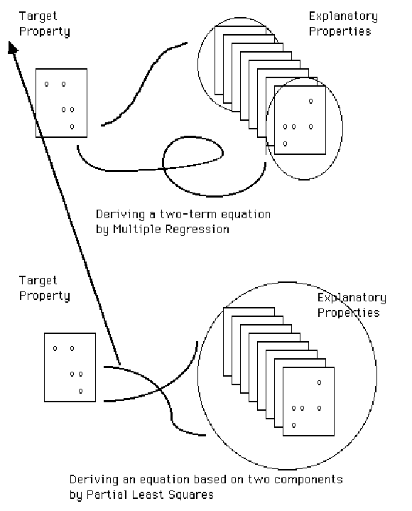
Another concern relates to the algorithmic mechanics of PLS. Why does MR consume one degree of freedom per explanatory column, but PLS generates many coefficients while consuming just one degree of freedom? Figure 24 provides some insight into the two processes. Both MR and PLS attempt to maximize overlap between target and explanatory properties. The difference is that MR maximizes the overlap of individual explanatory properties, one at a time, to extract a single coefficient. Each new column uses a degree of freedom, or row. PLS, on the other hand, maximizes overlap of the entire matrix of explanatory properties in each step. Because the entire matrix is always involved, extraction of a single PLS component generates a non-zero coefficient for every explanatory variable. Each new component also uses up a degree of freedom, or row, and when all possible components have been extracted, the coefficients generated by PLS are identical to those generated by MR. However, the model which is optimal with PLS often differs from that produced by MR because the crossvalidation criterion often prefers a PLS model with fewer than the maximum number of components.

Another way of describing PLS is to think of a factor analysis of the explanatory properties in which the objective is to maximize alignment with the target property values rather than with the Cartesian (or other) axes. For this reason PLS is sometimes likened to Principal Components Regression (PCR) a technique in which the scores from principal components analysis (PCA) are used in conventional MR. But, as detailed below, our view is that PCR is an inherently less efficient way of trying to accomplish the same thing as PLS.