4.5.6.1 Scope of Hierarchical Cluster Analysis
As in all multivariate analyses, the most important success factor in hierarchical clustering is relevant column property values. For hierarchical clustering in particular, the properties ought to be similar in kind and in numerical scale. Properties whose values differ most numerically tend to dominate the course of the analysis.
Hierarchical clustering makes heavy demands on computation. Both memory and processing time increase as the square of the number of rows in the original table. However, the effect of additional columns is much less severe.
A small example of the use of hierarchical clustering is given below. The following portion of a larger table was submitted for cluster analysis:
        TITLE:  bcdef
                                   1         2         3
                                  ActCo      LogP        MR
                               --------- --------- ---------
         1 Methane                -1.43      0.80      6.58
         2 Ethane                 -1.31      1.81     11.27
         3 Propane                -1.46      2.36     15.96
         4 n-Butane               -1.58      2.89     20.63
         5 2-Methylpropane        -1.68      2.76     20.85
         6 n-Pentane              -1.71      3.23     25.27
         7 2,2-DimethylPropane    -1.95      3.11     25.73
         8 2,2-DimethylButane     -1.90      3.82     29.94
         9 Cyclopentane           -0.88      3.00     23.14
        10 Cyclohexane            -0.90      3.44     27.71
The hierarchical clustering analysis was invoked with the following standard settings. At each invocation these tailor settings may be changed.
        Subject:   TAILOR!HIER

        Option Name         Description                             Value
        -----------         -----------                             -----

        CLUSTERING_METHOD   Method for determining cluster centers  SINGLE
        INPUT_FORM          Whether to compute distances            NORMAL_TABLE
        MOD_ANGLES          Whether to assume periodic variables    NO

        Dendrogram was calculated.
        Name for analysis> sample
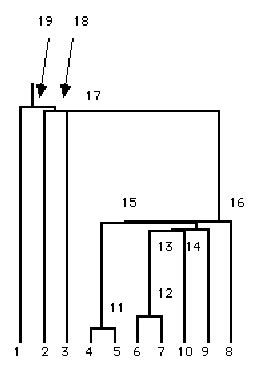
As with most SYBYL/QSAR analyses, results are automatically saved with the table for later study. The most complete and concise output is the graphical dendrogram, shown for this example as Figure 25, produced by MSS: QSAR >>> Graph QSAR (QSAR ANALYSIS GRAPH). Here is shown the textual output produced by MSS: QSAR >>> Report QSAR (QSAR ANALYSIS LIST).
        Cluster Node Membership

         #                  Methane  Ethane  Propane  n-Butane  2-Methylpropane
         -                  -------  ------  -------  --------  ---------------
         1 Cluster Level 1        1       2        3         4                5
         2 Cluster Level 2        1       2        3         4                4
         3 Cluster Level 3        1       2        3         4                4
         4 Cluster Level 4        1       2        3         4                4
         5 Cluster Level 5        1       2        3         4                4
         6 Cluster Level 6        1       2        3         4                4
         7 Cluster Level 7        1       2        3         4                4
         8 Cluster Level 8        1       2        3         3                3
         9 Cluster Level 9        1       2        2         2                2
        10 Cluster Level 10       1       1        1         1                1
         #                  n-Pentane 2,2-DimethylPropane 2,2-DimethylButane
         -                  --------- ------------------- ------------------
         1 Cluster Level 1          6                   7                  8
         2 Cluster Level 2          6                   7                  8
         3 Cluster Level 3          6                   6                  8
         4 Cluster Level 4          6                   6                  8
         5 Cluster Level 5          6                   6                  8
         6 Cluster Level 6          4                   4                  8
         7 Cluster Level 7          4                   4                  4
         8 Cluster Level 8          3                   3                  3
         9 Cluster Level 9          2                   2                  2
        10 Cluster Level 10         1                   1                  1

         #                  Cyclopentane Cyclohexane
         -                  ------------ -----------
         1 Cluster Level 1             9          10
         2 Cluster Level 2             9          10
         3 Cluster Level 3             9          10
         4 Cluster Level 4             9           6
         5 Cluster Level 5             6           6
         6 Cluster Level 6             4           4
         7 Cluster Level 7             4           4
         8 Cluster Level 8             3           3
         9 Cluster Level 9             2           2
        10 Cluster Level 10            1           1
As always, the initial cluster level has each row alone in a cluster, and the final level has all rows combined into a single cluster. Reading horizontally, we see that the first clustering (at Cluster Level 2) joins rows 4 and 5. Reading vertically, we see that ethane joins another cluster at the next to last level and methane survives alone until the end.
        Cluster Nodes Above Individual Rows

         #            Left-son Clusters Right-son Clusters
         -            ----------------- ------------------
         1 Node 10+1                  4                  5
         2 Node 10+2                  6                  7
         3 Node 10+3                 12                 10
         4 Node 10+4                 13                  9
         5 Node 10+5                 11                 14
         6 Node 10+6                 15                  8
         7 Node 10+7                  3                 16
         8 Node 10+8                  2                 17
         9 Node 10+9                  1                 18
        10 Node 10+10                19                  0

        Connection levels

        Level11   Level12   Level13   Level14   Level15   Level16   Level17
        -------   -------   -------   -------   -------   -------   -------
          0.274     0.533     2.265     2.298     2.438     2.473     4.702
        Level18   Level19   Level110
        -------   -------   --------
          4.725    4.799      5.251
These two listings indicate the cluster formations as they are graphed in the dendrogram. The first clustering of rows 4 and 5 occurs at a fairly low connection level (0.274), with rows 6 and 7 joining next. The third cluster level forms by joining Node 12 with Node 10, i.e. the cluster of rows 6 and 7 is joined to row 10. At almost the same connection level (vertical level on the dendrogram) we see the next cluster forming between the one just formed (Node 13) and row 9.
        Setup  : HIERARCHICAL CLUSTERING Analysis
          Minimum Sigma to use Column:  0.0000   Missing Values: DROP_ROW
          Clustering Method: SINGLE_LINKAGE   Input Form: NORMAL
          No distances were periodic.
          Columns
           1: ActCo                 2: LogP                  3: MR
          Rows (10 rows)
           1: Methane               2: Ethane                3: Propane
           4: n-Butane              5: 2-Methylpropane       6: n-Pentane
           7: 2,2-DimethylPropane   8: 2,2-DimethylButane    9: Cyclopentane
          10: Cyclohexane
The exact description of the analysis is also available in the listings.
Figure 25 Dendrogram of hierarchical clustering example.

The dendrogram is the primary result of most hierarchical clustering analyses. In Figure 25 the rows corresponding to each node in the treelike graph have been noted. Normally the graph consists of the lines only, and the Pick Points function (TABLE EXAMINE) is used to investigate cluster membership. In some cases, however, connection levels do not increase monotonically, and the relationships between clusters cannot be represented in this way. Warning: The Median clustering method will often produce such analyses, so that no dendrogram can be constructed.
The analyses are still valid and can be worked with through analysis listing as described above. Such analyses can also be output as cluster columns in the Advanced CoMFA module, but cannot be graphed as dendrograms.
Dendrograms can be used in at least two ways: to see which compounds are most similar in terms of the distance metric chosen, and to select a subset of compounds which are representative of the larger data set.
Here the most similar compounds cluster together at the lowest levels. Thus the most similar pairs are rows 4 and 5, and rows 6 and 7. The compounds in rows 1, 2 and 3 are somewhat similar to each other but quite different from the others. This is mainly due to the strong differences in MR for those rows as seen in the table listing above.
If the goal was to select 3 compounds of the 10 for more detailed study, it would be reasonable to select one compound from each of the top three levels. The top level contains row 1 and rows 2-10, so row 1 would be selected. The second level contains row 2 and rows 3-10, so row 2 is selected. And one compound from the remaining set would be needed, perhaps row 10.
The usefulness of the clustering is dependent on careful choice of the columns used, which determines the distances on which clustering operates.
Cluster columns are another powerful tool for working with cluster analyses. In the simplest case, such a column simply indicates which cluster each row belongs to at a specified level of clustering. The numbering of the clusters in this case, however, do not in general say anything about the relationship between clusters.
More information from a dendrogram can be captured in a cluster column by coordinating the numbering of clusters across several levels, so that low-level clusters which are related at higher levels bear cluster ID numbers which are close to one another. This happens to be the case in the listings given above: clusters 4-9 at cluster level 2 are all included in cluster 4 at cluster level 6. This introduces a partial order into the clustering which is useful for many graphing applications.


Copyright © 1999, Tripos Inc. All rights
reserved.


